Table of contents¶

1. Circular primes
   1. Prolog introduction and logical primality tests
   2. Translating satisfiable conditions
   3. Bringing it all together
   4. A technical note on implementation
2. Futoshiki
   1. Representing the game board
   2. Prolog arithmetic
   3. Solving Futoshiki
   4. Testing the solution
3. NYT Digits
   1. Prolog arithmetic, part two
   2. Solving Digits
4. Conclusion

Circular primes¶

The above riddle is an example of a constraint satisfaction problem (CSP), a special type of problem in which variables that have domains must be allocated values to satisfy some set of constraints. In the case of this particular riddle, we could model the 14 positions on the circle as variables $x_0,x_1,\dots,x_{13}$ (where we consider $x_{13}$ and $x_0$ to be neighbors), and the domain for each variable would be the integers 1–14.

The puzzle essentially boils down to two constraints on the variables: (1) each number from 1–14 must be used exactly once, and (2) the sum and difference of every pair of adjacent numbers must be prime. With these two constraints in mind, we can work toward building a general solver for the problem.

Prolog introduction and logical primality tests¶

First, we'll need a way to identify primes. Prolog is a logic programming language, so it operates with predicates instead of functions — predicates are statements about some input(s) that either hold or don't hold. One way of testing primality in Prolog can be achieved via the following:

%% is_prime(+N)
%
% Holds if N is a prime.

is_prime(2) :- !.
is_prime(3) :- !.

is_prime(N) :-
  N > 3,
  N mod 2 =\= 0,
  is_prime(N, 3).
is_prime(N, X) :-
  ( X*X > N ->
    true
  ; N mod X =\= 0,
    M is X + 2,
    is_prime(N, M)
  ).

And while the goal of this post is to demonstrate Prolog — not teach it — I recognize some background is still necessary, so the following will hopefully serve as a whirlwind tour of Prolog:

Firstly, there are two main ways of interfacing with Prolog: facts/rules, and queries. Facts and rules determine what can be queried, and they define expressions either declaratively or implicitly, respectively. For example, married(bob, john). is a fact declaring Bob to be married to John. An example of a rule could be is_single(Person) :- not(married(Person, _) ; married(_, Person)). which says that a person is single if they are not married to someone else (we need to account for both positions/relations in the married fact). Similar to a wildcard, the underscore indicates any person (we assume people cannot marry themselves).

Predicates are defined with the syntax head :- body. which reads as "the predicate head holds if body holds." And the body of a predicate consists of clauses linked by conjunctions ("and"s with a comma ,), disjunctions ("or"s with a semicolon ;), and are ended with a period .. Variables begin with uppercase letters, and constants (called atoms) begin with a lowercase. When we write is_prime(2) :- !. in the above code, we assert is_prime holds for the number two (or, that the number 2 is prime). The ! (called a cut) makes this subtly different, but we'll get to that shortly.

Querying in Prolog lets you interact with the "database" you've built from facts and rules/predicates. For example, if we query

?- is_single(john).
false.

we see that John is not single — i.e., he is married to someone. Now, let's say we want to find out who is married to whom. Since we know John isn't single, let's write a query for his spouse:

?- married(john, Person) ; married(Person, john).
Person = bob.

Person in the query is a variable (indicated by its uppercase starting character). Prolog shows us what Person was bound to in order to satisfy the query — in other words, if you "plug in" the result from Prolog, your query will evalute to true. You can think of it like Prolog saying: "here's what needs to be true for the query to hold." Note that here we have to write the married/2 relation twice to account for john being in either position in married/2.

If there are multiple ways to satisfy a query, Prolog will enumerate all possibilities. We can demonstrate this by adding another partner for John with the fact married(john, sam).:

?- married(john, P) ; married(P, john).
P = sam ;
P = bob.

This is a good time to mention that Prolog's inference engine features backtracking, which means it will generate multiple pathways for an execution to follow, pursue one, and then follow up on any paths that could satisfy the query later. In the above query, pressing ; will search for further satisfying bindings, and . will terminate the search.

Hopefully this brief primer gives you some intuition for the primality test code above. Some additional useful syntax to know is that ( X -> Y ; Z ) is an if-then-else block (if X then Y else Z), and predicates can share names as long as they have different arity (number of predicate arguments), which is typically written after the predicate name with a forward slash, e.g. is_prime/1 and is_prime/2.

Translating satisfiable conditions¶

Now that we can test for prime numbers, we need a predicate to determine whether the sum and difference of two numbers are prime:

%% prime_sumdiff(+N, +M)
%
% Holds if the sum and difference of N and M are both primes.

prime_sumdiff(N, M) :-
  Sum is N + M,
  Diff is abs(N - M),
  is_prime(Sum),
  is_prime(Diff).

This one is pretty simple: it takes two numbers N and M, computes their sum and difference (in Prolog, is evaluates an expression), and only holds if both are prime.

Next, to iteratively place our numbers in a circle, we can represent positions as a list, placing numbers left-to-right and ensuring that the last and first numbers also meet the prime sum-difference condition. While there are many ways to approach this, here's a recursive definition of the problem:

• Base case: all numbers have been placed correctly except for the last one, which must "fit" with $x_{n-2}$ and $x_0$ (the penultimate and first numbers)
• Recursive case: we must place some number $x_i$ next to the previous number $x_{i-1}$ while satisfying the prime sum-difference condition, and then place any remaining numbers

We can translate this into a predicate place_adjacents/3, starting with the base case:

%% place_adjacents(+Nums, -Placements, +Acc)
%
% Places each number in a list Nums into a circular list Placements in which
% each pair satisfies the prime sum-difference condition.

% base case
place_adjacents([N], Placements, [First|Acc]) :-
  last(Acc, Last), % need to place the last number
  prime_sumdiff(Last, N),
  prime_sumdiff(N, First),
  append([First|Acc], [N], Placements).

At a high level, this predicate takes the last number of our list of numbers to place, and ensures it meets the prime sum-difference condition with the first and last elements of the list-so-far before appending the number to the list-so-far, yielding the solution.

We can use Prolog's pattern matching to indicate that this predicate is only applicable when the first argument is a singleton list (with the last number N to place), meaning the predicate will only ever be used during the base case. Placements is the final placement list, and [First|Acc] is the list of digits so far with First being the first element (head) of the list and Acc the rest (tail) (in Prolog, the pipe character | is the construct operator).

We can similarly model the recursive case as:

% recursive case
place_adjacents(Nums, Placements, Acc) :-
  select(N, Nums, Nums1), % select the number to place
  last(Acc, Last),
  prime_sumdiff(Last, N),
  append(Acc, [N], Acc1),
  place_adjacents(Nums1, Placements, Acc1).

Which uses the built-in select/3 predicate to retrieve $x_i$ (N) from the available numbers Nums, leaving us with one less number in Nums1. Then, we compare $x_{i}$ with $x_{i-1}$ and add it to our list if it's compatible. To place the remaining digits, we recurse. Note that select/3 is used because it is "nondeterministic" and selects any number from our list of numbers to place.

Bringing it all together¶

With the bulk of the solver done, we need to "glue" our predicates together to create a simple interface. One implementation quirk we need to be careful of is that $x_{i-1}$ always exists in the recursive case (i.e. the accumulated list is never empty), so we need to ensure our main predicate begins with a number in the list (keeping in mind that it doesn't matter which number we start with, since a circular list has no "start" or "end").

%% circular_primes(+Low, +High, -Placements)
%
% Pairs numbers in a range [Low, High] such that the sums and differences of
% adjacent pairs of numbers in a circular list Placements are primes.

circular_primes(Low, High, Placements) :-
  Low < High,
  bagof(N, between(Low, High, N), Nums),
  select(First, Nums, NewNums), % select the first candidate number
  place_adjacents(NewNums, Placements, [First]).

This predicate accepts a valid lower and upper bound such that $\forall i:x_i\in\left[\verb|Low|,\verb|High|\right]$. Here, bagof is used to take all unique N such that N is between Low and High, storing the list in Nums (this specific usage of bagof is similar to Python's range() function). We also initialize the placement list with First, and state that in order for circular_primes/3 to hold, we must be able to place the remaining numbers NewNums as well.

And that's it! All that's left is to enter query mode and ask Prolog:

?- circular_primes(1, 14, Ps).
Ps = [1, 4, 7, 10, 13, 6, 11, 8, 3, 14, 9, 2, 5, 12] .

With the numbers 1–14, the predicate succeeds with the above placement specification. If we ask Prolog to keep generating solutions, we yield all of the different "rotations" or "shifts" (and reflections) of the circular list (for this example, there is only one unique solution):

?- circular_primes(1, 14, Ps).
Ps = [1, 4, 7, 10, 13, 6, 11, 8, 3, 14, 9, 2, 5, 12] ;
Ps = [1, 12, 5, 2, 9, 14, 3, 8, 11, 6, 13, 10, 7, 4] ;
Ps = [2, 5, 12, 1, 4, 7, 10, 13, 6, 11, 8, 3, 14, 9] ;
Ps = [2, 9, 14, 3, 8, 11, 6, 13, 10, 7, 4, 1, 12, 5] ;
Ps = [3, 8, 11, 6, 13, 10, 7, 4, 1, 12, 5, 2, 9, 14] .

And the best part is, since we've written a general solver for this type of question, we can ask Prolog for solutions for any range of numbers:

?- circular_primes(6, 24, Ps). % this has no solution
false.

?- circular_primes(6, 23, Ps).
Ps = [6, 11, 8, 15, 22, 19, 12, 7, 10, 21, 16, 13, 18, 23, 20, 9, 14, 17] .

A technical note on implementation¶

Before continuing, a brief note on alternative approaches — feel free to skip this part.

A natural question for a Prolog programmer at this point may be "Why not use CLP(FD)?" After all, this problem can (very easily) be described in the following two predicates:

1. $\forall i \forall j : x_i,x_j\in\left[1,14\right]\wedge x_i\ne x_j$
2. $\forall i : \text{Prime}\left(x_i+x_{(i+1)\bmod 15}\right)\wedge\text{Prime}\left(\left|x_i-x_{(i+1)\bmod 15}\right|\right)$

so why would would CLP(FD) not be the right approach?

The answer is: because of primality tests. Testing for primality is trivial when a variable is ground (e.g. in the above code), but primality is difficult to express as a constraint. This thread is the only working solution I've been able to find for a primality constraint, but the complexity is far beyond my level.

I was able to get a version using CLP(FD) working, but the performance is awful (I suspect due to the primality constraint). It's a shame, because the rest of the solution is extremely idiomatic:

%% place_clpfd(+Low, +High, -Placements)
%
% Pairs numbers in a range [Low, High] such that the sums and differences of
% adjacent pairs of numbers in a circular list Placements are primes.

place_clpfd(Low, High, Placements) :-
  % predicate 1 - variables in range and unique
  Len #= (High + 1) - Low, Len > 0,
  length(Placements, Len),
  Placements ins Low..High,
  all_distinct(Placements),

  % predicate 2 - sum-difference property
  sumdiff_clpfd(Placements), % for adjacent numbers
  Placements = [H | _],
  last(Placements, Last),
  sumdiff_clpfd([H, Last]),  % for first & last
  label(Placements).

%% sumdiff_clpfd(+List)
%
% Holds if the sum and differences of all adjacent numbers in List are primes.

sumdiff_clpfd([]).
sumdiff_clpfd([_]).
sumdiff_clpfd([N, M | T]) :-
  Sum #= N + M,
  Diff #= abs(N - M),
  prime(Sum),
  prime(Diff),
  sumdiff_clpfd([M | T]).

But finding the solution to the simple 1–14 puzzle yields, in comparison to the vanilla Prolog solution:

?- time(place_clpfd(1, 14, Ps)).
% 1,100,236 inferences, 0.053 CPU in 0.053 seconds (99% CPU, 20840171 Lips)
Ps = [1, 4, 7, 10, 13, 6, 11, 8, 3, 14, 9, 2, 5, 12] .

?- time(circular_primes(1,14,Ps)).
% 3,673 inferences, 0.000 CPU in 0.000 seconds (97% CPU, 17743961 Lips)
Ps = [1, 4, 7, 10, 13, 6, 11, 8, 3, 14, 9, 2, 5, 12] .

...yep. The accumulator solution above (which I'm confident is inefficient) uses ~300x less inferences than the CLP(FD) one. It's possible a more efficient primality constraint exists out there, or it's possible I'm doing something totally wrong — either way, if you have any information surrounding this, please let me know!

Futoshiki¶

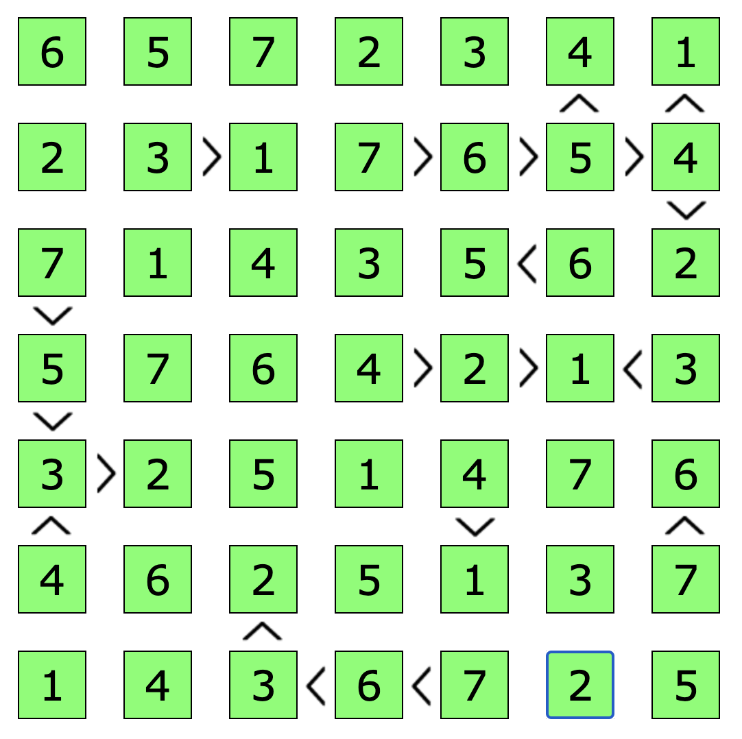
Futoshiki (不等式) is a logic puzzle game about inequalities. Each puzzle grid is a $n\times n$ board with optional starting numbers, and given inequality symbols ($<$ and $>$). A solved puzzle is a Latin square where the digits $1$ to $n$ appear exactly once in each column and row, similar to Sudoku. The twist is that digits within cells must also satisfy any surrounding inequalities. Refer to the image below for an example:

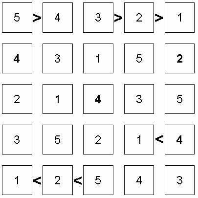
Futoshiki is a fantastic game because it requires chains of deductive inference (e.g. "this square can't be X because cell Y has to be larger than cell Z") — I fully encourage you to try a few games.

From an objective point of view, though, Futoshiki is just another constraint satisfaction problem: we want to slot the numbers $1$–$n$ in unique board positions such that the Latin square property holds and all inequalities are satisfied. Since we can define the game in terms of properties that should be true in a solved state, we can try implementing a solver in Prolog!

Representing the game board¶

For the $n\times n$ grid, we'll use the standard approach of nested arrays — but we still need a way to represent inequalities on the board with respect to different squares. One way of doing this is to specify an array of (row, col) pairs and describe the relationship between them. In the above example board, we can represent the inequality on the fourth row as (4,4)<(4,5) if we use one-based indexing and define (1,1) to be the top-left cell.

To use this approach, we'll first have to tell Prolog that we're reserving the < and > characters for our own purposes (as part of a grammar representing an inequality):

:- op(650, xfy, <).
:- op(650, xfy, >).

Which just overrides Prolog's default behavior of < and >. Now, we'll define a predicate to tell us whether or not an inequality in our format holds:

%% constraint_holds(+Grid, +Constraint)
%
% Holds if Constraint, indicated by (Row1,Col1)<|>(Row2,Col2), is true
% within the Grid.

constraint_holds(Grid, (R1,C1)>(R2,C2)) :-
  nth1_matrix(R1, C1, Grid, Elem1),
  nth1_matrix(R2, C2, Grid, Elem2),
  Elem1 #> Elem2.
constraint_holds(Grid, (R1,C1)<(R2,C2)) :-
  nth1_matrix(R1, C1, Grid, Elem1),
  nth1_matrix(R2, C2, Grid, Elem2),
  Elem1 #< Elem2.

These two predicates do the same thing, but using < and > means we need to specify pattern matches for both symbols (as far as I can tell — if you know a way around this, please reach out). In both predicates, we're simply navigating to Grid[R1][C1] and asserting it is strictly less than or greater than Grid[R2][C2], accordingly.

This nth1_matrix/4 is a helper-predicate to access a 2D array, and can be defined as follows:

%% nth1_matrix(?Row, ?Col, +Matrix, ?Elem)
%
% Way to access Row-th row and Col-th column of Matrix. Holds if
% Matrix[Row][Col] is Elem.

nth1_matrix(Row, Col, Matrix, Elem) :-
  nth1(Row, Matrix, MatRow),
  nth1(Col, MatRow, Elem).

Prolog arithmetic¶

You may have picked up on the weird #< and #> operators in constraint_holds/2. Explaining this requires some understanding of math in Prolog: in Prolog, arithmetic is fairly straight forward: let's say we want to check the parity of the integer X:

?- X = 10, X mod 2 =:= 0.
X = 10.

We simply set X to 10 and check if $x \bmod 2$ is zero, using =:= for evaluated expression equality. Numerical constraints, on the other hand, are not so straight forward: doing any comparison on arithmetic-bound variables requires those variables to be instantiated. For example, if we wanted to find every even integer between zero and ten:

?- X > 0, X < 10, X mod 2 =:= 0.
ERROR: Arguments are not sufficiently instantiated
ERROR: ...

While you might expect this to yield 2, 4, and so on, we instead get an error. This is because in order to evaluate X mod 2, X needs to be bound, but we don't know the exact value of X when we need to instantiate it — so we get a sort of circular problem. To circumvent this, we can use the CLP(FD) library for numeric constraints by including it in our file:

:- use_module(library(clpfd)).

Which defines the operators #=, #<, #>, and so on for constraint definitions. Then, we can retry our original query using the new operators:

?- X #> 0, X #< 10, X mod 2 #= 0.
X in 2..8,
X mod 2#=0.

This may look strange, but this is CLP(FD) at work — to turn this expression into bound variables, we have to label/1 the data:

?- X #> 0, X #< 10, X mod 2 #= 0, label([X]).
X = 2 ;
X = 4 ;
X = 6 ;
X = 8.

This is why #< and #> are used in our constraint_holds/2 predicate — because we want to put constraints on variables we don't know the values of yet. The possibilities with CLP(FD) and its accompanying CLP(Z) library are quite endless — see here for more.

Solving Futoshiki¶

Although specifying inequalities in the format (R1,C1)<|>(R2,C2) works, chains of inequalities become clumsy: for example, (R1,C1)<(R2,C2)<(R3,C3) is represented by [(R1,C1)<(R2,C2), (R2,C2)<(R3,C3)], meaning we have to duplicate the intermediary cell (R2,C2).

We can remedy this by creating a predicate that breaks down such chains into their constituents:

%% decompose_ineqs(+Expr, -Dec)
%
% Decomposes a string of inequalities (in the form (Row1,Col1)(<|>)(Row2,Col2))
% into a list of separate inequalities, e.g. A<B>C -> [A<B, B>C].

decompose_ineqs(Expr, Dec) :- decompose_ineqs(Expr, [], Dec).
decompose_ineqs(Expr, Acc, Dec) :-
  ( Expr = A<B<C ->
    append(Acc, [A<B], Acc1),
    decompose_ineqs(B<C, Acc1, Dec)
  ; Expr = A>B<C ->
    append(Acc, [A>B], Acc1),
    decompose_ineqs(B<C, Acc1, Dec)
  ; Expr = A<B>C ->
    append(Acc, [A<B], Acc1),
    decompose_ineqs(B>C, Acc1, Dec)
  ; Expr = A>B>C ->
    append(Acc, [A>B], Acc1),
    decompose_ineqs(B>C, Acc1, Dec)
  ; Expr = A<B ->
    append(Acc, [A<B], Dec)
  ; Expr = A>B ->
    append(Acc, [A>B], Dec)
  ).

This looks like it's doing a lot because of exhaustive pattern matching, but really, it's just breaking down long expressions of inequalities into pairs of expressions our constraint_holds/2 predicate can validate. For example:

?- decompose_ineqs((R1,C1)<(R2,C2)<(R3,C3), Constituents).
Constituents = [(R1, C1)<(R2, C2), (R2, C2)<(R3, C3)].

With this functionality, we are now in a pretty good position to solve a generic Futoshiki puzzle:

%% solve_futoshiki(+Grid, +Constraints)
%
% Solves a Futoshiki board where the grid is a square 2D array of arrays, and
% constraints to satisfy are supplied as an array.

solve_futoshiki(Grid, Constraints) :-
  % constraint 1 - Latin square
  length(Grid, Rows), maplist(same_length(Grid), Grid), % square grid
  append(Grid, Values), Values ins 1..Rows, % all values between [1,n]
  maplist(all_distinct, Grid), % rows all different

  % cols
  transpose(Grid, Cols),
  maplist(all_distinct, Cols), % cols all different

  % Constraint 2 - inequalities are satisfied
  maplist(decompose_ineqs, Constraints, IneqsList),
  append(IneqsList, Ineqs),
  maplist(constraint_holds(Grid), Ineqs),
  maplist(label, Grid).

First, we ensure the Latin square properties hold: (1) the grid is square (the number of columns are equal to the number of rows); (2) the values in the grid all fall within $[1,n]$; and (3) each number appears in each row and column exactly once (we use CLP(FD)'s all_distinct/2 to ensure all rows/cols are different).

The inequalities in the grid can be validated by (1) decomposing all supplied inequalities and creating a single inequality list; and (2) mapping over this list and ensuring all constraints hold in the grid. And that's it! Relatively straightforward when defined at a high-level like this, so let's try it out on some puzzles.

Testing the solution¶

We'll start with an easy 4x4:

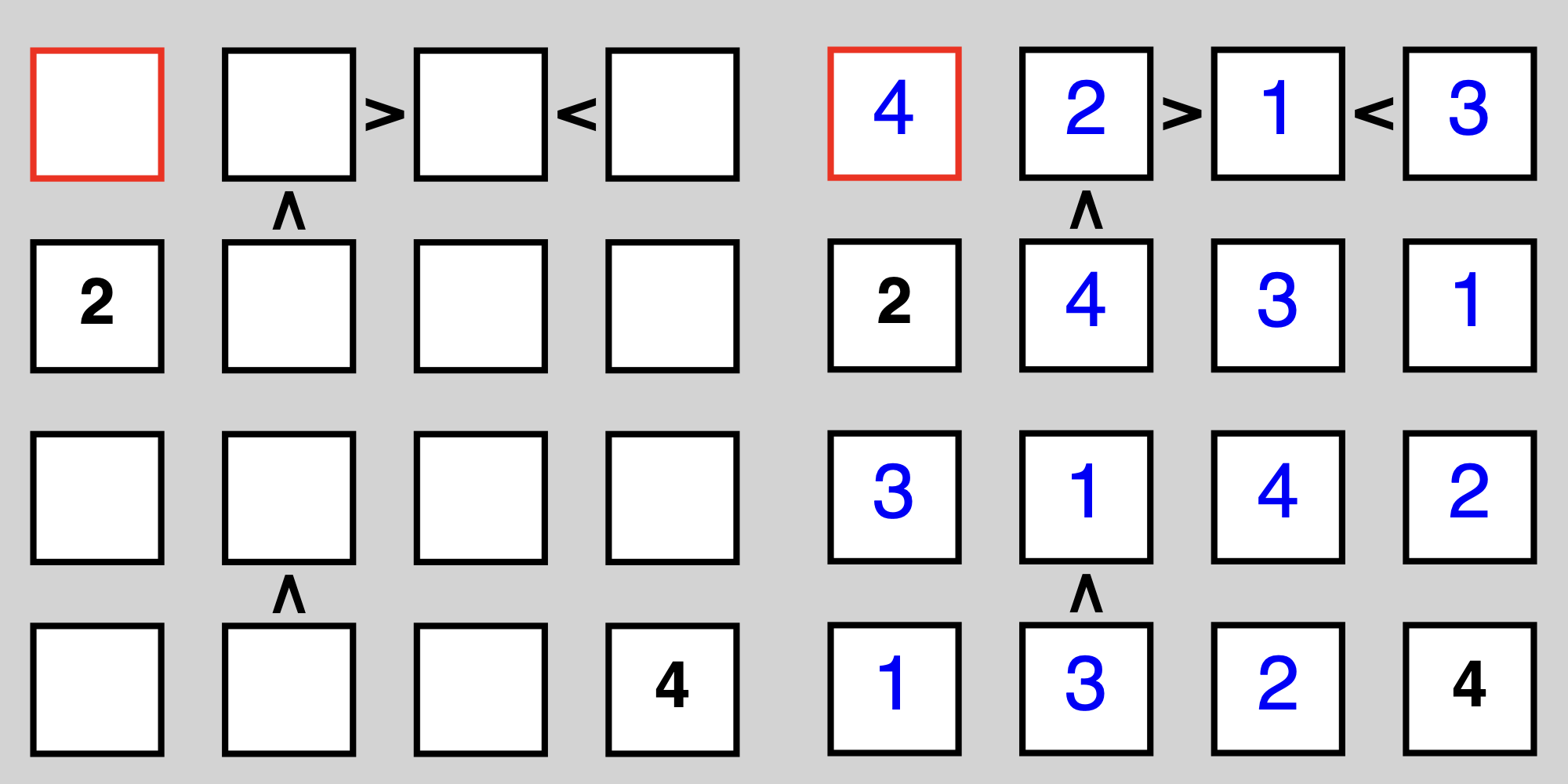
For our predicate, we represent empty cells with unbound logic variables in a $4\times4$ nested array (with 2 and 4 supplied). We also supply the two chains of inequalities like so:

test(1) :-
  Grid = [
    [_, _, _, _],
    [2, _, _, _],
    [_, _, _, _],
    [_, _, _, 4]
  ],
  Constraints = [
    (2,2)>(1,2)>(1,3)<(1,4),
    (4,2)>(3,2)
  ],
  solve_futoshiki(Grid, Constraints),
  write(Grid).

And query the result via:

?- test(1).
[[4,2,1,3],[2,4,3,1],[3,1,4,2],[1,3,2,4]]
true .

Here's another example with a more difficult 7x7:

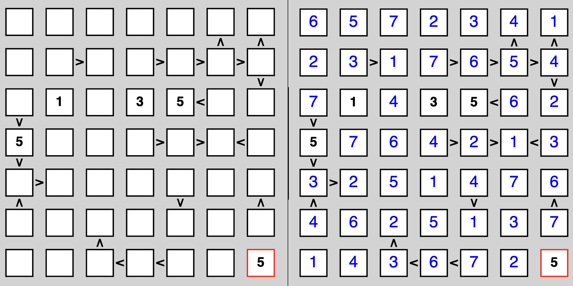
A 7x7 grid is annoying to type, so here I just implicitly define the grid and instead set given digits with our indexing predicate:

test(2) :-
  length(Grid, 7),
  maplist(same_length(Grid), Grid),
  nth1_matrix(3, 2, Grid, 1),
  nth1_matrix(3, 4, Grid, 3),
  nth1_matrix(3, 5, Grid, 5),
  nth1_matrix(4, 1, Grid, 5),
  nth1_matrix(7, 7, Grid, 5),
  Constraints = [
    (2,2)>(2,3),
    (2,4)>(2,5)>(2,6)>(2,7)>(3,7),
    (2,6)>(1,6),
    (2,7)>(1,7),
    (3,1)>(4,1)>(5,1)<(6,1),
    (5,1)>(5,2), (3,5)<(3,6),
    (4,4)>(4,5)>(4,6)<(4,7),
    (5,5)>(6,5), (5,7)<(6,7),
    (6,3)<(7,3)<(7,4)<(7,5)
  ],
  solve_futoshiki(Grid, Constraints),
  write(Grid).

For fun, let's see how long Prolog takes to solve this:

?- time(test(2)).
[[6,5,7,2,3,4,1],[2,3,1,7,6,5,4],[7,1,4,3,5,6,2],[5,7,6,4,2,1,3],[3,2,5,1,4,7,6],[4,6,2,5,1,3,7],[1,4,3,6,7,2,5]]
% 407,146 inferences, 0.032 CPU in 0.034 seconds (96% CPU, 12554223 Lips)
true .

Taking roughly 0.034 seconds and half a million logical inferences (what does this mean?).

Prolog's nondeterminism also means that puzzles with multiple solutions solve correctly (Prolog can enumerate all of them). The following puzzle has two solutions, which our solver identifies:

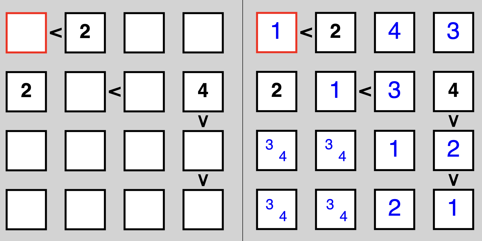
test(6) :-
  Grid = [
    [_, 2, _, _],
    [2, _, _, 4],
    [_, _, _, _],
    [_, _, _, _]
  ],
  Constraints = [
    (2,4)>(3,4)>(4,4),
    (1,1)<(1,2),
    (2,2)<(2,3)
  ],
  solve_futoshiki(Grid, Constraints),
  write(Grid).

Since the 3-4 pair can be in either location, Prolog identifies the two configurations:

?- test(6).
[[1,2,4,3],[2,1,3,4],[3,4,1,2],[4,3,2,1]]
true ;
[[1,2,4,3],[2,1,3,4],[4,3,1,2],[3,4,2,1]]
true ;
false.

And that's a small and simple Futoshiki solver. If you're interested in looking at the source code in one place, my efforts are available on Github.

NYT Digits¶

From April 10th to August 8th 2023, the New York Times published daily puzzles for a game they called Digits, a math puzzle game. They've since discontinued the game (I guess it didn't have enough consistent players), but luckily it still lives on in good old internet fashion.

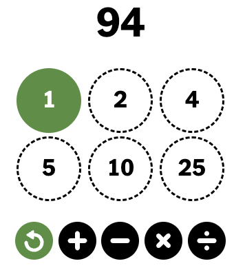
In Digits, players are given a set of six numbers of which they have to apply the four arithmetic operations to (add, subtract, multiply, divide) in order to produce a target integer. Once used in an operation, two numbers create a new number, and you cannot reuse the old numbers. For example, the above puzzle has the solution $(4\times 25) - (1+5) = 100 - 6 = 94$.

At first blush, this game might seem impossible to translate into a Prolog solver, because it's unclear how predicates might come into play. However, approaching the problem from a "grammatical" viewpoint can make it easier to frame as a recursive problem:

Every solution to a Digits puzzle is an number derived from an expression, which itself is a combination of two expressions, and so on. We can enumerate the rules like so:

which, for example, allows us to visualize the derivation of the solution:

Understanding how Prolog deals with expressions in this format is important to solving Digits, so one last detour before the solution:

Prolog arithmetic, part two¶

Earlier in this post I mentioned "evaluating" expressions using the is keyword, but what does this really mean? In Prolog, variables assigned arithmetic expressions are not immediately evaluated — for example:

?- X = 5, Y = 10 - 5.
X = 5,
Y = 10-5.

in any other language, you would probably expect something like Y = 5., but Prolog instead binds the variable to the expression that yields five.

Prolog also ensures no order-of-operations trickery happens when combining expressions, as it automatically adds parentheses to expressions:

?- X = 7-2, Y = 10, Z = Y - X.
X = 7-2,
Y = 10,
Z = 10-(7-2).

Once variables hold expressions, we can evaluate them to yield the values:

?- X = 7-2, Y = 10, Z = Y - X, Val is Z.
X = 7-2,
Y = 10,
Z = 10-(7-2),
Val = 5.

So why is this relevant, and how can we use this to solve Digits?

Solving Digits¶

The recursive nature of Digits and the grammar of arithmetic expressions means we can loosely form a naïve search strategy:

• Base case: the expression we have constructed evaluates to the target number.
• Recursive case: from the set of available expressions (or integers), choose two and create a new expression via an arithmetic operation.

Put simply, choosing two different expressions and combining them in some way either yields our target number, or a new expression to use later. Let's implement this strategy from the top-down:

%% find_expr(+Available, +Cur, +Target, -Expr)
%
% Searches for an expression Expr using terms in Available that equals Target.
% Stores current accumulated expression in Cur.

find_expr(Available, Cur, Target, Expr) :-
  ( Cur =:= Target ->
    Expr = Cur
  ; % otherwise, take two from available
    select(E1, Available, A1),
    select(E2, A1, A2),
    transform_expr(E1, E2, NewExpr),
    NewAvailable = [NewExpr | A2],
    find_expr(NewAvailable, NewExpr, Target, Expr)
  ).

First, we tell Prolog that if our current expression Cur evaluates to Target, we should stop the search and bind to the expression Expr. In the recursive case, we take two expressions E1 and E2 from the current pool of expressions and combine them in some way, before adding the new expression to the pool and recursing.

Of course, we now need a way to transform two expressions:

%% transform_expr(+Expr1, +Expr2, -NewExpr)
%
% Enumerates all ways to combine two expressions Expr1 and Expr2 with the four
% operations of arithmetic, yielding a new expression NewExpr.
transform_expr(Expr1, Expr2, NewExpr) :-
  ( 
    NewExpr = Expr1 + Expr2 ;
    NewExpr = Expr1 - Expr2 ;
    NewExpr = Expr1 * Expr2 ;
    NewExpr = Expr1 / Expr2 
  ),
  EvalNewNum is NewExpr,
  EvalNewNum > 0,
  integer(EvalNewNum).

This is where Prolog's representation of arithmetic comes in handy: Prolog essentially has the grammar we defined earlier built into it, not only allowing us to combine expressions with ease, but storing expressions in variables means we don't have to do any fancy backtracking to trace solution derivations.

The above predicate simply takes two expressions, and says that a "transformed" new expression NewExpr combining the two must use one of the four arithmetic operations and must also result in a positive integer (when evaluated). That's it — for completeness, I'll define a final predicate as an interface to write the results:

%% solve_digits(+Nums, +Target)
%
% Solves the NYT game "Digits" by taking in a list of available starting
% numbers Nums, and a target number Target.

solve_digits(Nums, Target) :-
  find_expr(Nums, 0, Target, Expr),
  format('~w~25| = ~w~n', [Expr, Target]).

Which produces the solution to the above example:

?- time(solve_digits([1,2,4,5,10,25], 94)).
(1+2+10)*5+4+25           = 94
% 145,950 inferences, 0.008 CPU in 0.008 seconds (100% CPU, 17575867 Lips)
true .

And does so in less than 0.01 seconds. It also solves the hardest puzzle of the last day the game was playable:

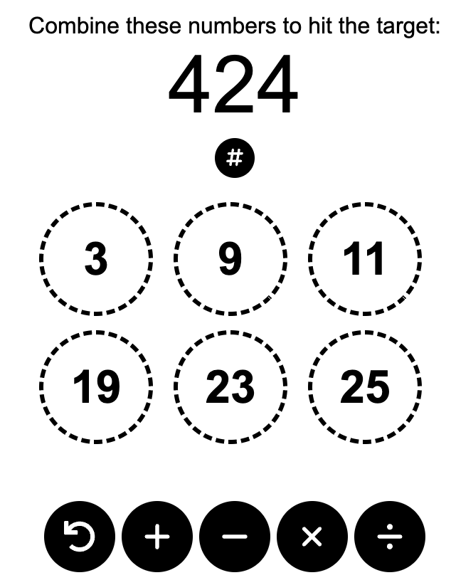
?- time(solve_digits([3,9,11,19,23,25], 424)).
23*25-((3+9)*11+19)       = 424
% 72,163 inferences, 0.011 CPU in 0.011 seconds (98% CPU, 6792451 Lips)
true .

...in about half the inferences!

Conclusion¶

None of the above three puzzles are particularly challenging or computationally difficult. They could be solved in other languages, but the point is that Prolog was designed exactly for the kind of problems exhibited in this post, and it really shows. Modeling problems in Prolog feels satisfying, regardless of whether implementations are rough and inefficient (like in the circular primes problem), or well-defined systems of constraints (like in Futoshiki).

There is also a practical incentive for using Prolog: more often than not, modeling CSPs or other problems in Prolog just makes sense — why should I go to the trouble of building my own backtracking or dynamic programming algorithm for every scenario I face, when I could benefit from Prolog's inference engine and great libraries like CLP(FD)/CLP(Z)?

Hopefully this post has given you a reason to try out a new language, or at least share some appreciation of an awesome tool lesser-known to the common programmer.